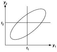
One assumption of the tetrachoric and polychoric correlation coefficients is underlying bivariate normality: that the pre-discretized, latent versions (y1 and y2) of your variables, of which your observed measures (x1 and x2) are dichotomous or ordered-category manifestations, have a bivariate normal distribution.

This assumption is not as limiting as it might appear. It is actually only necessary that some monotonic transformation of y1 and y2 exists, such that the transformed versions have a bivariate normal distribution, a milder assumption.

In any case, there are probably instances where, for empirical or theoretical reasons, latent bivariate normality is not plausible; then the assumption can be relaxed. For this, we make use of a convenient identity between (a) the tetrachoric/polychoric corelation model and (b) the latent trait model (Lazersfeld & Henry, 1968; Bock & Lieberman, 1970; Bock & Aitkin, 1981).

Takane & de Leeuw (1987) demonstrate that the latent bivariate normal model of the tetrachoric/polychoric correlation is isomorphic with and identically equalivant to the latent trait model with a normally distributed latent trait. That is, the two models portrayed below are equivalent:

Figure 1a. Tetrachoric correlation model: bivariate normal distribution of two latent continuous variables (y1 and y2) and discretizing thresholds (t1 and t2).		Figure 1b. Latent trait model with two dichotomous manifest variables and a normally distributed latent trait.

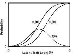
Both models will equally well predict observed data, and the parameters of one are algebraically translatable to those of the other.

Figure 1b shows a latent trait model for a pair of dichotomous variables. There, f (θ) is the pdf of a latent trait θ common to a pair of variables; θ here is assumed to have a normal (Gaussian) distribution.

p₁(θ) and p₂(θ) are the response functions for the two variables. In a rater agreement analysis, these are the probabilities (for rater 1 and rater 2, respectively), of the rater making a positive rating given a case with each possible latent trait level. If measurement error for both raters is assumed to be Gaussian and heteroscedastic (i.e., constant variances across levels of θ ), then the response functions have the forms of normal cdfs. The integrals used to solve the model in Figure 1b then involves simple convolutions of normal distributions, and are equivalent to the integration of the bivariate-normal distribution in Figure 1a. Thus we can estimate the tetrachoric/ polychoric correlation coefficient using either model and get the same results.

Moreover we may exploit this correspondance to generalize the tetrachoric/polychoric correlation coefficient. The latent trait distribution in Figure 1b need not be normal. It can have any shape -- for example, skewed. A skewed normal latent trait distribution would correspond to a pear-shaped distribution in Figure 1a.

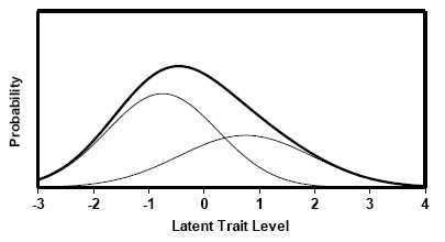Figure 2. Skewed latent trait distribution modeled as a mixture
of two normal distributions.

A convenient way to model a skewed latent trait distribution is as a mixture of two component normal distributions (Figure 2). To estimate latent correlation in a 2×2 table, one would need to specify the parameters of this mixture a priori. However with a 3×3 or larger table, the optimal mixture parameters can be estimated from the observed data.

Thus, by means of a latent trait model with a skewed or non-normal latent trait distribution, one may estimate various generlizations of the tetrachoric/polychoric correlation coefficient. The following programs can be used for this:

• The glc program (generalized latent correlation) estimates the latent correlation for pairs of dichotomous variables with a user-specified skewed latent trait distribution; it is very easy to use.

• The LTMA program (latent trait mixture analysis) can be used to estimate latent correlation in a 3×3 or larger table. One can specify the shape of the latent trait distribution in advance or let the program estimate it. The analytic model is described by Uebersax & Grove (1993). The current program version can be a little awkward to use.

• The LLCA program (located latent class analysis). Again for 3×3 or larger tables. This is like the LTMA program except that it uses a non-parametric model for the latent trait distribution: the distribution is modeled as a set of locations or nodes along the x-axis (vis-a-vis Figure 1b); the density of the distribution at each node is then estimated. The model is described in Uebersax (1993). This program, like the LTMA program, is not recommended for inexperienced users.

  Note that the LTMA and LLCA programs can also estimate latent agreement among 3 or more raters simultaneously; in this case, you would be performing a latent trait analysis proper.

Bock RD, Aitkin M. Marginal maximum likelihood estimation of item parameters: application of an EM algorithm. Psychometrika, 1981, 46, 443-459.

Bock RD, Lieberman M. Fitting a response curve model for dichotomously scored items. Psychometrika, 1970, 35, 179-198.

Lazarsfeld PF, Henry NW. Latent Structure Analysis, Boston: Houghton Mifflin, 1968.

Lord FM, Novick MR. Statistical Theories of Mental Test Scores. Reading, Massachusetts: Addison-Wesley, 1968.

Takane Y, de Leeuw J. On the relationship between item response theory and factor analysis of discretized variables. Psychometrika, 1987, 52, 393-408.

Uebersax JS. Statistical modeling of expert ratings on medical treatment appropriateness. Journal of the American Statistical Association, 1993, 88, 421-427.

Uebersax JS, Grove WM. A latent trait finite mixture model for the analysis of rating agreement. Biometrics, 1993, 49, 823-835.

Last updated: 6 Febrary 2008